Introduction
A solar model is the solution to a set of equations describing the physical processes occurring within the Sun. These equations are often divided into two subsets, the structure equations and the chemical evolution equations. In the very simplest cases, these equations are coupled nonlinear first-order ordinary differential equations, but more realistic models usually involve coupled nonlinear first-order partial differential equations. In either case, the equations cannot be solved analytically and thus must be solved numerically. Therefore, a solar model is usually comprised of a set of tables describing the conditions (chemical composition, density, luminosity, mass, pressure, temperature, etc.) at different depths in the star.
Equations of Stellar Structure
The physical variables involved in these equations are luminosity, mass, pressure, radius, and temperature. Other quantities such as density, energy generation rate, and opacity, are derived from these five variables. The equations of stellar structure are usually written with mass as the independent variable, not radius. One reason for this is that most stellar models assume that the star has constant mass over a given time but not constant radius. Indeed, we expect the radius of a star to vary over its lifetime.
The equations of stellar structure in my model are
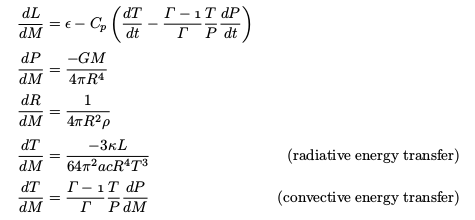
where L is the luminosity, M is the mass, P is the pressure, R is the radius, T is the temperature, t is the time, ε is the energy generation rate (from nuclear fusion), κ is the Rosseland mean opacity, and ρ is the density. Other physical constants have their usual meanings.
Equations of Chemical Evolution
The equations of chemical evolution depend solely upon which nuclear processes are running in the interior of the star. In the Sun, the most important fusion process is the proton-proton chain (pp chain) which fuses four hydrogen atoms to one helium atom. However, another reaction network called the carbon-nitrogen-oxygen cycle (CNO cycle) is also active in the Sun, although it is much less important than the pp chain. In my model I keep track of five elements: hydrogen, two species of helium, carbon, and nitrogen. After making certain simplifying assumptions, the equations of chemical evolution in my model are
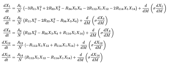
where RIJ is the reaction rate between species I and species J, X1 is the hydrogen abundance, X3 is the helium 3 abundance, X4 is the helium 4 abundance, X12 is the carbon 12 abundance, X14 is the nitrogen 14 abundance, and σ is a collection of constants which includes a diffusive term.
The total abundance (the sum of all the abundances) must equal one so each abundance is a number between zero and one.
Energy Generation
The energy generation rate can be described by something as simple as a power law to more complicated expressions involving nuclear reaction rates. My more advanced solar model uses the equation

Opacity
Like the energy generation rate, opacity can be described by a power law but more complicated models use opacity tables. I use the OPAL opacity tables and then perform a four-dimensional interpolation procedure across the logarithms of the hydrogen abundance, metals abundance, density, and temperature.
Density
For the purposes of my model, the ideal gas equation of state is used in the calculation of density.

The variable μ is the mean molecular weight and Z is the metals abundance (not including carbon 12 or nitrogen 14).
Convection and Overshooting
Because no theory of convection exists, the problem of convective versus radiative transport of energy is treated very simply. The Schwarzschild condition is used to determine whether the radiative or convective transport derivative is used for each calculation. The amount of overshooting past the edge of any convective zone is handled simply: a percentage of the mass of the convective zone. The more overshooting there is, the longer the initial convective core lasts.
Diffusion
A very simple diffusion function is used. The diffusion constant is taken to be a very large value in convective regions and zero in radiative regions. The diffusion function is
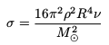
where ν is the diffusion constant.
Other Considerations
Effects from magnetism, rotation, and non-sphericity are not considered.
Boundary Conditions
The central boundary conditions for the stellar structure equations are taken to be
- L = 0
- P = Pc (central pressure)
- T = Tc (central temperature)
The central pressure and temperature are unknown and their values must be estimated. The surface boundary conditions for the stellar structure equations are taken to be
- L = Ls (surface luminosity)
- P = 0
- R = Rs (surface radius)
- T = 0
Again, the surface luminosity and radius are unknown and their values must be estimated.
For the chemical evolution equations, the diffusion is taken to be zero at the centre and surface.
Initial Conditions
The initial conditions that need to be specified are the initial chemical abundances, and estimates for the central pressure and temperature, and surface luminosity and radius. A homogeneous chemical abundance distribution is the most usual configuration. My model begins with a homogeneous distribution of
- X1 = 0.71
- X3 = 0.00001
- X4 = 0.27
- X12 = 0.2 Z
- X14 = 0.05 Z
where Z = 1.0 − X1 − X3 − X4.
Procedure for Calculating a Solar Model
For a given set of initial conditions, the equations of stellar structure are solved to give a model at a given time. Once the model has been calculated, the chemical abundances are evolved one time step. Then a new model can be calculated for the evolved chemistry. This new model is then used to improve the chemical abundances for that time step and a final model for the given time step is calculated. This predictor-corrector procedure continues until the desired age of the star is reached.
Singularities at the Centre and Surface
It is clear that for the given boundary conditions, the equations of stellar structure are singular at both the centre and the surface. Therefore, it is necessary to use special techniques at both boundaries to safely integrate away from them. My model uses truncated series approximations to the solutions at the centre and surface.
Numerical Algorithm
The two-point boundary value problem involving the equations of stellar structure is solved using a shooting method. My ordinary differential equation integrator is the classical fourth-order Runge-Kutta algorithm. The initial model is calculated using adaptive stepsize control so that the mass grid has a fine mesh near the centre and the surface. (The adaptive scheme is related to the scale heights of the four physical variables.) Since the integrator cannot be used at the centre or the surface, special routines described above are used to take the first step out from the centre and in from the surface. The shooting method involves integrating out from the centre and in from the surface to some fitting point. If the correct values for central pressure and temperature, and surface luminosity and radius have been used, then the values for luminosity, pressure, radius, and temperature will agree at the fitting point for both integrations. However, if the values do not agree, a multidimensional Newton-Raphson method is used to find the corrections to the unknown boundary conditions that will hopefully improve the fit. This process of “shooting”, comparing the fit, and correcting the boundary conditions continues until the values agree at the fitting point.
Technically, the luminosity equation is not an ordinary differential equation but a partial differential equation when entropy terms are included. The time derivatives are simply written as backward differences.
The evolution equations are nonlinear partial differential equations. The nuclear source terms are linearized according to the scheme
XIk+1∙XJk+1 − XIk+1∙XJk + XIk∙XJk+1 − XIk∙XJk
where k denotes the time step and I and J denotes the species. When diffusion is included, tridiagonal systems result for each species. The evolved value of helium 3 is solved for first, followed by carbon 12. Nitrogen 14 is calculated next in such a way as to guarantee that the total abundance of carbon 12 and nitrogen 14 is constant. Finally, the hydrogen abundance is computed. Helium 4 is obtained by subtracting the known quantities from one. Once approximations for the new abundances are known, the equations are solved again and again until the improvement is negligible. Only then is the next model calculated.